Laser Measurements 101
Part 6: A BOGO Special
A Buy One Get One sale (BOGO) is the best friend of the girl math inclined! Today, it’s also the best friend of the laser measurements inclined. I’m going to explain how we can make two measurements simultaneously. We’re not talking about sequential measurements, or using two different lasers. We can actually measure two completely independent quantities – distance and velocity as you may have guessed – from a single data set!

It may sound impossible to measure two unrelated quantities using a single measurement, but it is merely extremely difficult. In fact, there are only a few sensor technologies in wide use that can do this at all:
- Nitrogen-vacancy center sensors measure magnetic field and temperature
- Microwave resonant sensors measure thickness and dielectric permittivity
- Ellipsometers measure thickness and refractive indices of thin films.
Each of these has something in common with our self-mixing laser setup: they use the frequency response of waves. As we’ve discussed in the prior parts, we will continue to do the same.
Remember that we can measure velocity by maintaining our laser at a constant power, measuring the frequency of our laser photodiode. The velocity is given by the equation:
$$ v = \lambda \frac{\Delta f}{2}$$

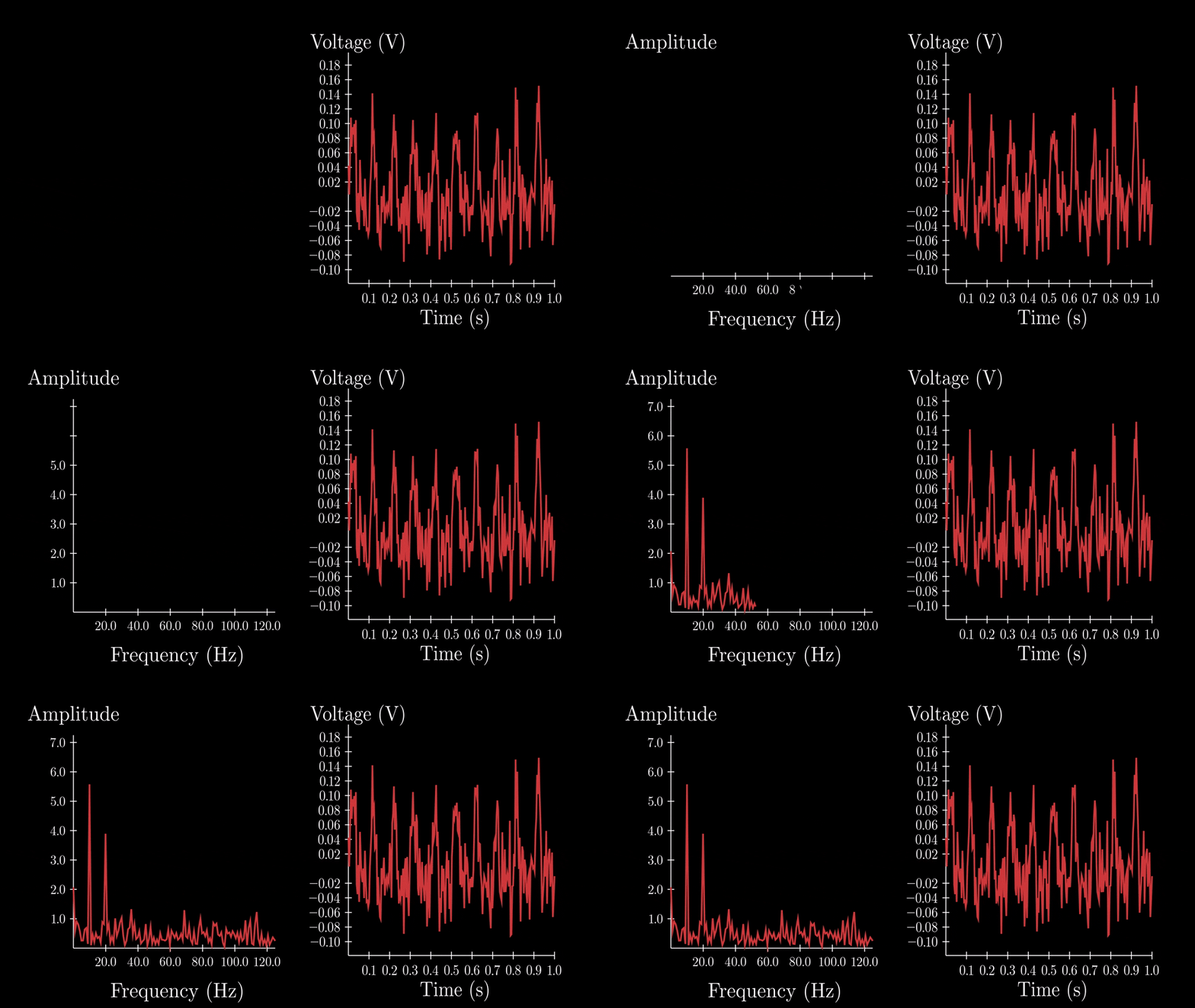
We measure this by recording the voltage of the photodiode and taking the FFT to get a frequency spectrum.
Here you can see what this looks like. Of course, the time would be much shorter than the axis shown. Often the measurement would happen in milliseconds or even \(\mu s \). It’s important that it happens quickly so that the distance and velocity aren’t changing significantly during the measurement.
As you can see, the FFT will have a spike at the main frequency induced by the velocity, in this case at 10Hz. You’ll notice that there is also a spike at 20Hz, which is a “harmonic”, it’s like an echo of the primary frequency, and we’ll ignore it.
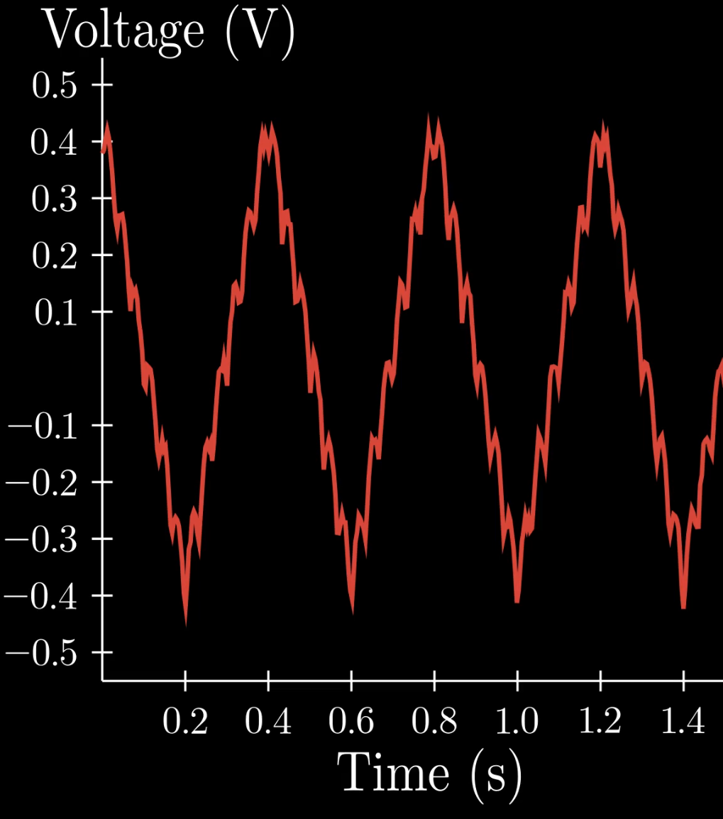
So we have a frequency measurement for velocity, and we can apply the same logic to distance! As you can see, and you remember from part 5, we are now modulating the brightness in a triangle shape. This causes the wavelength to change, which causes the smaller pulses to happen, and we take an FFT on this measurement to get those frequencies.


So what happens if we take an FFT of the modulated signal to get distance, but the target is also moving? For our purposes, lets assume that the distance is fixed, but there is a velocity.
An example of this case is we are measuring the speed of a feed of material like paper, measuring the speed of a treadmill, or a moving vehicle by pointing the laser at the ground.
In all of those cases, there is a distance to the object, and the speed of the object, and the two are independent from each other.
This animation shows the mechanic at work. You can see that if the target is moving towards the laser, and wavelength is decreasing, the two effects offset, and there are very few fringes!
The opposite also happens, as you can see in this second animation. If the target is moving towards the laser, and the wavelength increases, then there are twice as many fringes!
If we do an FFT on the demodulated and amplified signal, we see that the single peak we saw previously has now split into two peaks, one for each section of the modulation!
We can see from the animations that the single frequency becomes 2 frequency peaks. Why? Fascinatingly, the fringes have a sign. There are positive fringes – where the waves are jumping “forwards”, and negative fringes where the waves are jumping “backwards”. This means we can no longer just add and subtract frequencies however we like, because there are now positive and negative frequencies. The term for this which I find helpful to think of is phase stimulus. I will oversimplify here, and we will talk more on phase stimulus in the Laser Measurement 102 series!
Because the phase stimulus can be positive or negative, the frequency from velocity or distance can be positive or negative. However, the FFT only measures the real (read: positive) frequencies. So we can only measure the absolute value of the frequencies.
$$ f = |f_{distance}| \pm |f_{velocity}|$$
Where \(f_{distance}\) is the signed change in frequency due to the modulation, and \(f_{velocity}\) is the signed change in frequency due to the velocity of the target! The key term of course is the fat \(\pm\) obstructing our equation. This denotes that if the velocity and distance frequencies are moving together, they add. If they are moving apart, they subtract. You can see this in the previous animations. This will be our two frequencies we measure in the FFT \(f_1\) and \(f_2\)!
$$ f_1 = |f_{distance}| + |f_{velocity}|$$
$$ f_2 = |f_{distance}| – |f_{velocity}|$$
I spared you a derivation of this equation, but I’m sure you are wondering where the absolute values come from. The short answer is they come from solving a differential equation which results in a square root, and therefore the absolute value.
If we simply rearrange and solve the equations for for \(f_{velocity}\) and \(f_{distance}\), you get the following equations:
$$ f_{distance} = \frac{f_1 + f_2}{2} $$
$$ f_{velocity} = \frac{f_1 – f_2}{2} $$
This perfectly mirrors are prior experience from the animations! The frequencies stay centered on the \(f_{distance} \) value, and will spread out evenly based on the velocity. This makes sense, because when we had 0 velocity, the two frequencies were the same, and we only had one peak!
Now we just do this modulation, measure both frequency peaks, and we have both distance and velocity! Perfect.
The video below explains all of this in great detail, and also dives into our next upcoming blog topic: scale.
