Laser Measurements 101
Part 3: What About Distance?
When you think about measuring something with a laser, you likely think of either laser scanning, or LiDAR. In fact, there are at least 3 good ways of measuring distance, and each have their own advantages and disadvantages! We’ll walk through each of them, including my personal favorite at the end.
Method #1: LiDAR
Light Detection And Ranging (LiDAR) stole its name from Radar; Radio Detection And Ranging. However, the way it works is more like Sonar; Sonic Detection and Ranging!
We’ve all heard the pulses sent out by submarines in movies, and we understand that they wait to see how long it takes for the sound to bounce back, and that tells them the distance to objects.
LiDAR is the same idea, except unlike Radar and Sonar, it’s much easier to focus a laser into a narrow beam than radio or ultrasonic waves.
This narrower beam means we can measure many more points in space. In addition, the light-speed waves allows us to collect samples much faster than sound waves. Engineers are clever, and put the sensor on a spinning mount to take advantage of this!
From this, we can collect a very dense point cloud, more than 10 million points per second!
Any good economist will tell you there’s no such thing as a free lunch. Any good engineer will concur, there is always a tradeoff! In this case, LiDAR’s downside is poor performance for short distances.
For example, let’s say we want to have a lidar system which measures the time of flight down to the nearest 0.1 nanoseconds (100 picoseconds). Given the equation:
$$ d = v t $$
In this case, \(v = c\) where \(c\) is the speed of light at \(~300e^6\). So if we have an error of \(100e^{-9}\) seconds, that’s a distance error of 3cm. If we’re doing range finding for artillery and our measurement is 1km away, it’s only 0.003% error. Fantastic!
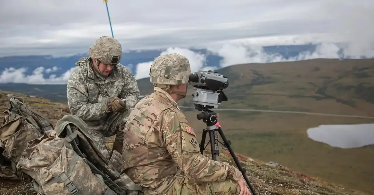
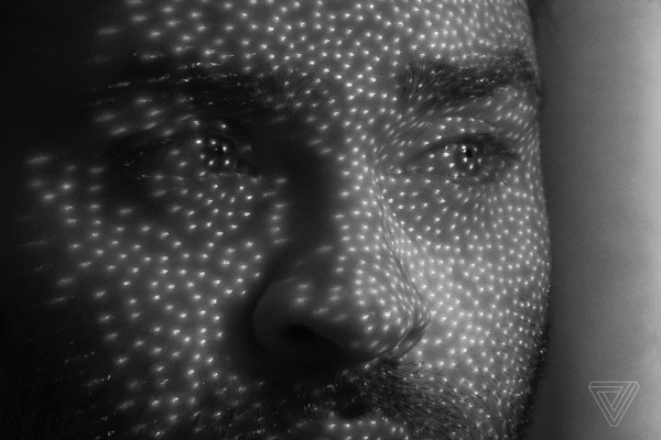
But if we want to laser scan an intricate part only 1 meter way, it’s 3% error, not so great. This is why LiDAR isn’t used for laser scanning, facial recognition, or other applications where distances are less than ~1 meter.
Instead, they use structured light to determine the shape from distortion patterns!
Method #2: Triangulation
The next way to measure the distance to an object using a laser is called “triangulation”. I’ll give you one guess which shape is involved!
This one is downright clever. Remember in part 1 we noted that a laser will scatter in all directions when it hits a (non-mirror) surface? We can use that to our advantage, and capture as much of that light as possible using a big lens.
Then, we’ll focus that light onto a single point onto a linear image sensor. A linear image sensor is essentially just an array of photodiodes in a straight line. Imagine a camera sensor but with only 1 row of pixels instead of many rows and columns.
Just as before, tradeoffs manifest immediately. This time in the need for the lens to focus the light and contrast it from the background ambient light. If you take a laser pointer outside on a sunny day, it looks quite dim, and it might disappear entirely to your eyes. We introduce extra complexity to overcome this issue, including a wavelength filter which only allows laser light through, or a clever modulation strategy must be implemented. This is in addition to the bunch of extra photodiodes, and extra lens we require beyond the LiDAR arrangement.
The accuracy is now only limited by the precision of the image sensor, so the short-range measurement is much more precise! This measurement method excels at precision distance measurement for short distances, and fails miserably in the same distances where LiDAR is perfectly suited! Likely for these reasons, these have been the 2 dominant distance measurement methods since the invention of laser sensing!
But there is a 3rd method which is gaining popularity, and even better – it can coexist with the velocity measurement strategy we discussed in part 2!
Method #3: Self Mixing
Previously, we discussed using a photodiode to measure the difference between the emitted and returned frequencies, and how that would allow us to measure velocity. Using some clever math, we can measure distance with an accuracy of 1 wavelength! The key is hidden in this equation:
$$ D = n \lambda$$
Don’t get scared by the Greek letter \(\lambda\), I know we’ve all been traumatized by the Greek alphabet, but stay calm. \(\lambda\) just means the wavelength of the wave! \(n\) is the number of periods, and \(D\) is the distance traveled.
Essentially, that equation is just the definition of a wave! So if we want to measure D, we just need to know n and \(\lambda\).
The problem is, we don’t know how many periods our wave has, so how does this help us? Let’s try a similar trick as for velocity, and use a change in values! Maybe that will be easier to measure! Note that at some distance, \(D = n_1 \lambda_1 \), and if \(\lambda_1\) changes to a new value \(\lambda_2\), then what happens to n? What will be the value of \(n_2\)? Simple, because D has not changed, the product of \(n \lambda\) must be conserved:
$$D = n_2 \lambda_2 = n_1 \lambda_1$$
Now, let’s make 2 assumptions.
First, we’ll assume we can coax the wavelength to change in a consistent way, so that \(\Delta \lambda\) is consistent. In other words, we don’t know what the values of \(\lambda_1\) or \(\lambda_2\) are, but we do know they aren’t changing, so the difference between them \(\Delta \lambda = \lambda_2 – \lambda_1\) is constant, and their ratio \(\frac{\lambda_1}{\lambda_2}\) is also constant. We’ll discuss how we can achieve this later, but for now, let’s assume we can make this happen.
Our second assumption is to assume that we can measure \(\Delta n = n_2 – n_1\). In fact, this will be our core measurement for how we know distance! We have no way to directly measure \(n_1\) or \(n_2\), but if we can measure their difference, that’s all we need!
We know that at a given distance, D, \(n_1\) and \(n_2\) both have values given by:
$$ n_1 = \frac{D}{\lambda_1}$$ $$n_2 = \frac{D}{\lambda_2}$$
And we know that we can measure \(\Delta n\) which is given by:
$$\Delta n = n_2 – n_1 = \frac{D}{\lambda_2} – \frac{D}{\lambda_1} = D ( \frac{1}{\lambda_2} – \frac{1}{\lambda_1} ) $$
Now let’s imagine that we moved to a new distance, \(D^{‘}\) which is some distance x times further away. In other words:
$$ D^{‘} = xD$$
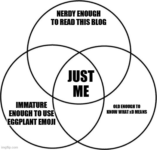
This could also be written as 🍆= 😆. And yes, I’m aware that the audience for that joke is ~1 person.
In any case, we want to see what the new value of \(\Delta n^{‘}\) will be, and we’re hoping that it will be something predictable so that our measurement of \(\Delta n\) will suffice as a measurement for distance! Let’s assume there are new values for \(n_1^{‘}\) and \(n_2^{‘}\). Using the same equations as before, we know that:
$$ n_1^{‘} = \frac{D^{‘}}{\lambda_1} = \frac{yD}{\lambda_1} $$
$$ n_2^{‘} = \frac{D^{‘}}{\lambda_2} = \frac{yD}{\lambda_2} $$
You can already see that this means \(\Delta n^{‘}\) is quite easily to calculate:
$$ \Delta n^{‘} = n_2^{‘} – n_1^{‘} = \frac{yD}{\lambda_2} – \frac{yD}{\lambda_1} = y \Delta n $$
How convenient! This means that for any distance we choose, the \(\Delta n\) will scale perfectly with distance! If this feels obtuse to you, don’t worry. This is a mathematical proof of a concept which I find easier to visualize. So I created a visualization in the video linked at the end of this blog post.
The takeaway is that if we can modify the wavelength \(\lambda\) in a consistent way, and measure the number of period changes \(\Delta n\) when we made those modifications, then we have a measurement that perfectly correlates with distance.
Note that we don’t have a scale yet. We know that if we double distance, our measurement doubles. If we cut distance in half, our measurement is cut in half. But we don’t know the actual value, until we measure \(\lambda\) and \(n\) at a known distance. So we’ll need to calibrate this measurement at some point when we know what the true distance is. After that, however, we can simply rely on measuring \(\Delta n\)
The next two blog posts will focus on how we can meet those two assumptions we made earlier:
- How can we modify the wavelength of a laser predictably and consistently?
- How can we measure the \(\Delta n\) directly?
If you are like me, your eyes glaze over when you read equations. That’s why I made a video illustrating these concepts in an intuitive visual way! Check it out below.